

sent on November 21, 2025
I’m always pumped when I get GPS data on a case. Shockingly though, about 50% of the time I end up with raw GPS coordinates that have to be processed to generate a speed trace. 100% of the time I forget how I’ve done it in the past.
After digging through some of my Harley Boom! Box research, several papers, and experimenting with a few tools, my memory is refreshed. Here’s what I’ve found.
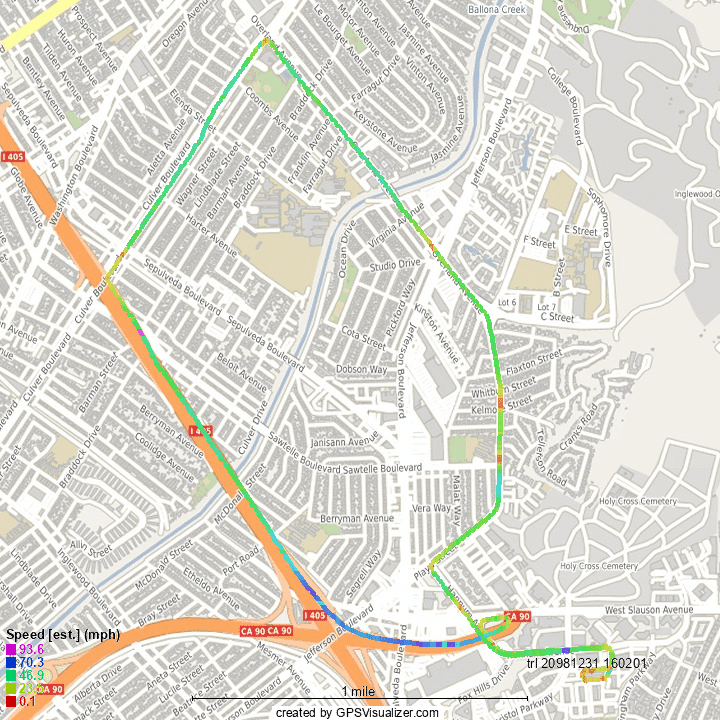
1: GPS Visualizer’s website won't win any design awards, but it works like a charm. You can upload data in various formats to visualize or convert it. I’m generally using this to go from a GPX file to raw text data I can bring into Excel, but experiment with the JPEG/PNG/SVG maps and you’ll find it makes great demonstratives too. Like this:
2: The Haversine formula is a user-friendly way to accurately calculate distances between coordinates. It looks like this, where μE is the mean radius of the Earth (credit to vcalc.com):

3: You’re 95% of the way there now, so halfway done. Once you get your timing into workable units, leg speeds can be calculated (D from above / time interval).
4: When you plot the result, you’ll likely see a lot of noise and a few outliers. I’ve found (as have others) that a 5-point moving average goes a long way to clean things up. The graph below shows a speed trace calculated from Harley Boom! Box data compared to VBOX speeds. The red is the unfiltered Harley data, the black is the 5-point average, and the blue is the VBOX. Not bad at all!

Some authors use more sophisticated filters, like the Kalman or Savitzky-Golay, but for typical vehicle speeds and low-frequency data (~1Hz), I’ve found the simple moving average works really well.
Thanks for reading along, have a great weekend and Thanksgiving. I’ll see you back here on December 5th!
Lou Peck
Lightpoint | JS Forensics
P.S. VLC recently crossed 6 billion downloads! The internet agrees, Jean-Baptiste Kempf (and his team) are heroes.